5. Interpreting the Results

In solving for coil paths, pyCoilGen generates the following output files:

• If debug is greater than 0, it produces some intermediate images.

• If save_stl_flag is True, it generates 3D .stl mesh files. By default, save_stl_flag is True.

• If skip_postprocessing is True, it skips computation of SolutionErrors. By default, skip_postprocessing is False.

5.1. Intermediate Images

If debug has a value greater than 0, pyCoilGen produces three PNG images with a filename derived from the project name as defined in project_name:

For example, for a project_name of ygradient_cylinder, the intermediate image files are:

• 10_ygradient_cylinder_0_5_contours_0_p.png: Shows the initial, open, contours paths.

• 14_ygradient_cylinder_0_5_contour_centres_0_p.png: Shows the closed contours with their contour group centres.

• 16_ygradient_cylinder_0_5_wire_path2_uv_0_p.png: Shows the fully joined wire path.

5.2. Output Meshes

If save_stl_flag is True, pyCoilGen generates two 3D .stl mesh files per detected coil part with a filename derived from the project name as defined in project_name.

For example, for a project_name of ygradient_cylinder, the .stl files are:

• ygradient_cylinder_surface_part0_y.stl : Shows the winding coil surface for the first coil part.

• ygradient_cylinder_swept_layout_part0_y.stl : Shows the 3D swept mesh of the winding coil conductor for the first coil part.

5.3. CoilSolution

The CoilSolution class is a data structure that contains all data loaded and processed by pyCoilGen. You can use this information to perform further analysis, especially of the solution_errors.

class CoilSolution:
    coil_parts: List[CoilPart]          # The processed CoilParts
    target_field: TargetField           # The computed TargetField
    combined_mesh: DataStructure        # A composite mesh constructed from all CoilParts meshes.
    sf_b_field: np.ndarray              # The magnetic field generated by the stream function.
    primary_surface_ind                 # Index of the primary surface in the of the coil_parts list.
    solution_errors: SolutionErrors     # The solution errors, if computed.

5.4. SolutionErrors

Unless skip_postprocessing is set to True, the SolutionErrors class contains information about the solution. You can use this information to evaluate the computed target field produced by the calculated coil wire path. This information is used by the plotting examples, below.

class SolutionErrors:
    """Maximum and mean relative errors."""
    field_error_vals: FieldErrors               # Detailed errors, by field
    combined_field_layout: np.ndarray           # Resulting target field by final wire path.
    combined_field_loops: np.ndarray            # Resulting target field by contour loops.
    combined_field_layout_per1Amp: np.ndarray   # Resulting target field by final wire path, for 1 A current.
    combined_field_loops_per1Amp: np.ndarray    # Resulting target field by contours loops, for 1 A current.
    opt_current_layout: float                   # The computed current that will achieve the desired target field.
    sf_b_field_1A: np.ndarray                   # The stream function field for 1 A current.
    target_field_1A: np.ndarray                 # The target field for 1 A current.

combined_field_layout contains the magnetic field vectors due to the final coil wire path.

combined_field_loops contains the magnetic field vectors due to the unconnected contour loops.

5.4.1. FieldErrors

The FieldErrors structure contains the maximum and mean relative errors for the computed solution, as percentages.

class FieldErrors:
    """Maximum and mean relative errors, in percent."""
    max_rel_error_layout_vs_target: float
    mean_rel_error_layout_vs_target: float

    max_rel_error_unconnected_contours_vs_target: float
    mean_rel_error_unconnected_contours_vs_target: float

    max_rel_error_layout_vs_stream_function_field: float
    mean_rel_error_layout_vs_stream_function_field: float

    max_rel_error_unconnected_contours_vs_stream_function_field: float
    mean_rel_error_unconnected_contours_vs_stream_function_field: float

The layout variables contain values computed due to the final wire path.

The unconnected_contours variables contain values computed due to the contour loops.

The vs_target variables contain values computed with respect to the provided target field.

The vs_stream_function variables contain values computed with respect to the computed stream function.

5.5. Visualising the Results

There are plotting routines in pyCoilGen.plotting that are useful for visualising the results.

5.5.1. Example Results: S2 Shim Coil

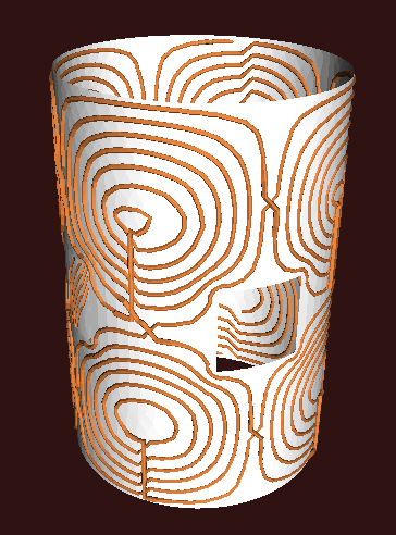
A 3D rendering of the .stl output for the s2_shim_coil_with_surface_openings.py example.

After running the s2_shim_coil_with_surface_openings.py example, the results can be saved to PNG files using the code below.

from os import makedirs

import matplotlib.pyplot as plt
from pyCoilGen.helpers.persistence import load
import pyCoilGen.plotting as pcg_plt

solution = load('debug', 's2_shim_coil', 'final')
which = solution.input_args.project_name
save_dir = f'{solution.input_args.output_directory}'
makedirs(save_dir, exist_ok=True)

coil_solutions = [solution]

# Plot a multi-plot summary of the solution
pcg_plt.plot_various_error_metrics(coil_solutions, 0, f'{which}', save_dir=save_dir)

# Plot the 2D projection of stream function contour loops.
pcg_plt.plot_2D_contours_with_sf(coil_solutions, 0, f'{which} 2D', save_dir=save_dir)
pcg_plt.plot_3D_contours_with_sf(coil_solutions, 0, f'{which} 3D', save_dir=save_dir)

# Plot the vector fields
coords = solution.target_field.coords

# Plot the computed target field.
plot_title=f'{which} Target Field '
field = solution.solution_errors.combined_field_layout
pcg_plt.plot_vector_field_xy(coords, field, plot_title=plot_title, save_dir=save_dir)

# Plot the difference between the computed target field and the input target field.
plot_title=f'{which} Target Field Error '
field = solution.solution_errors.combined_field_layout - solution.target_field.b
pcg_plt.plot_vector_field_xy(coords, field, plot_title=plot_title, save_dir=save_dir)

5.5.1.1. 2D Computed Stream Function and Contours

A colour plot showing the 2D stream function and the corresponding contour groups. This is computed by projecting the 3D coil mesh onto 2D.

This figure shows the target field stream function overlaid with the computed contours. The contour groups are shown in different colours.

5.5.1.2. The 3D Computed Stream Function and Contours

A 3D colour plot showing the stream function and the corresponding contour groups projected onto the coil mesh.

This figure shows the target field stream function overlaid by the computed contours. The contour groups are shown in different colours.

5.5.1.3. The Target Field Z-Component

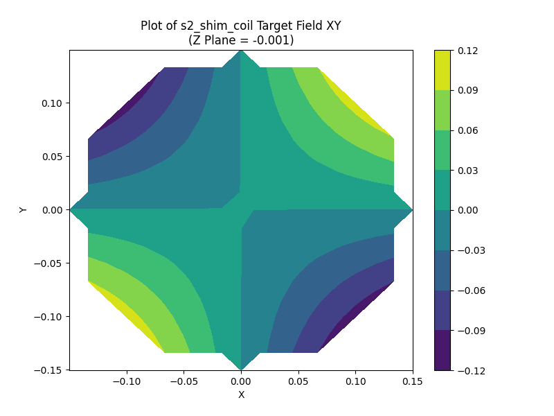
A colour plot of the Z-component of the target field vector in the X-Y plane at the mean Z-axis value.

This figure shows the value of the Z-component of the combined field due to the computed wire path.

5.5.1.4. The Target Field Z-Component Difference

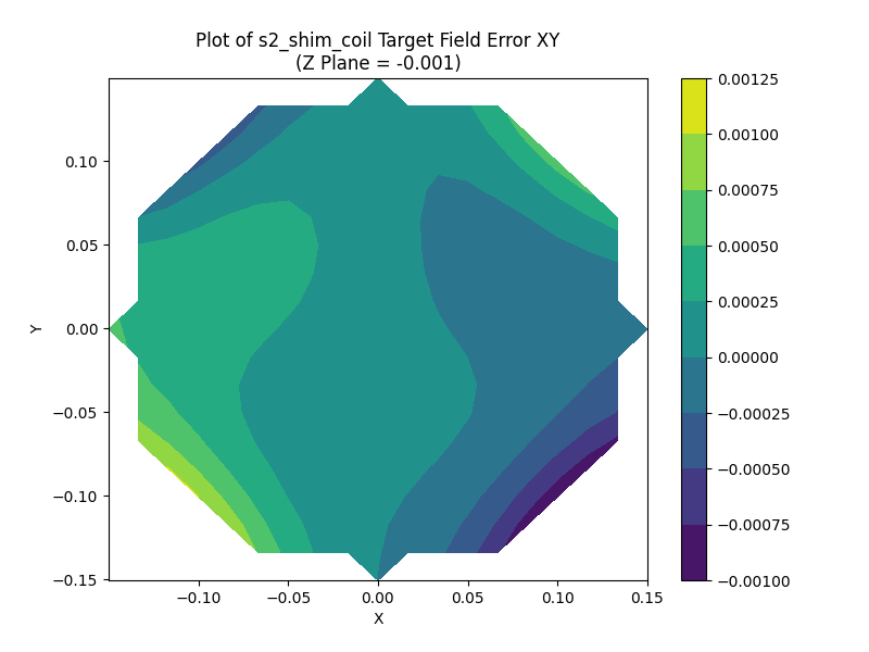
A colour plot of the Z-component of the relative error between the computed field and the input target field.

This figure shows the difference between the magnetic field vector and the specified target field in the X-Y plane, computed at the mean Z-axis value.

5.5.1.5. Summary of Fields and Errors

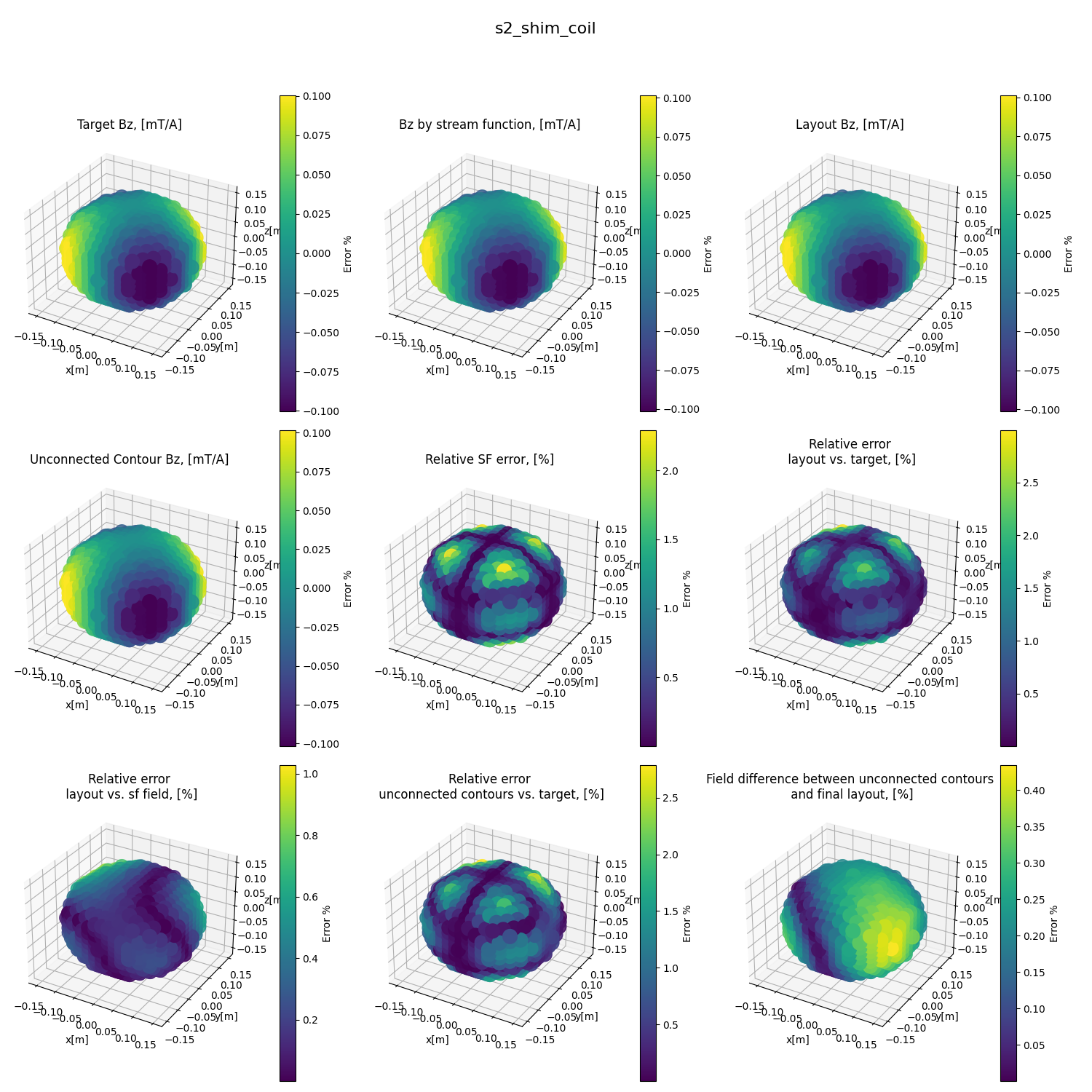
A multi-plot showing various views of the results for the s2_shim_coil_with_surface_openings.py example.

5.6. Visualising Multiple Solutions: A Parameter Sweep

The halbach_gradient_x.py example uses multiprocessing to do a sweep through two input parameters, tikhonov_reg_factor and levels.

This example also generates plots that summarise the key error parameters.

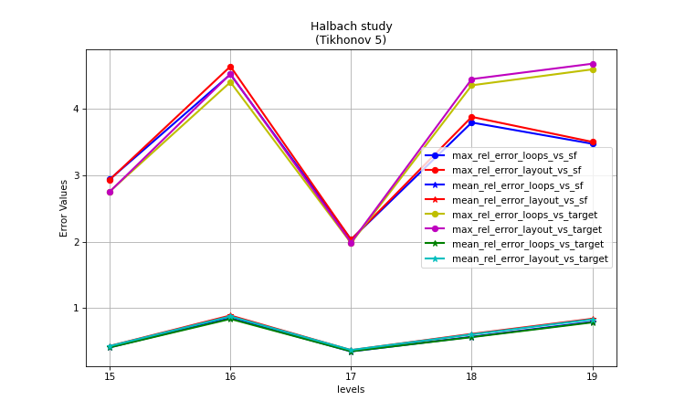
A plot showing the error metrics of the parameter sweep. This plot shows the effect of level on the error values, for tikhonov_reg_factor equal to 5.

A plot showing the error metrics of the parameter sweep. This plot shows the effect of level on the error values, for tikhonov_reg_factor equal to 10.

As can be seen in these two plots, there is a sweet spot at tikhonov_reg_factor=5 and levels=17.